
Libration
Presentation and Results
The Moon exhibits an oscillatory motion around its principal axis, with an amplitude of about 7 degrees, called longitudinal libration.
In the traditional SM (Spinning Moon) conception, this phenomenon is explained kinematically, through the combination of the eccentricity of the lunar orbit and its supposed rotation on its own axis.
In the NSM (Non‑Spinning Moon) conception, where this rotation does not exist, libration can be explained as the conjunction of two dynamical effects:
- the well‑known tidal effect 1, presented for example in https://en.wikipedia.org/wiki/Tidal_locking
- a previously unstudied effect, which we call the tumble effect2, which would be caused by a slight mass imbalance in favor of the hemisphere facing the Earth.
¹ In NSM the tidal effect is real, although synchronous rotation is not.
2 The tidal and tumbling effects both result in a pendulum-like movement.
The program, whose source code is provided below, can be run in two modes: a main mode called “libration”, and an auxiliary mode called “rotation”.
Thanks to the Matplotlib library, the image of the Moon is added to the plot at regular angular intervals, and the final image at the end of the orbit is produced at the end of the program.
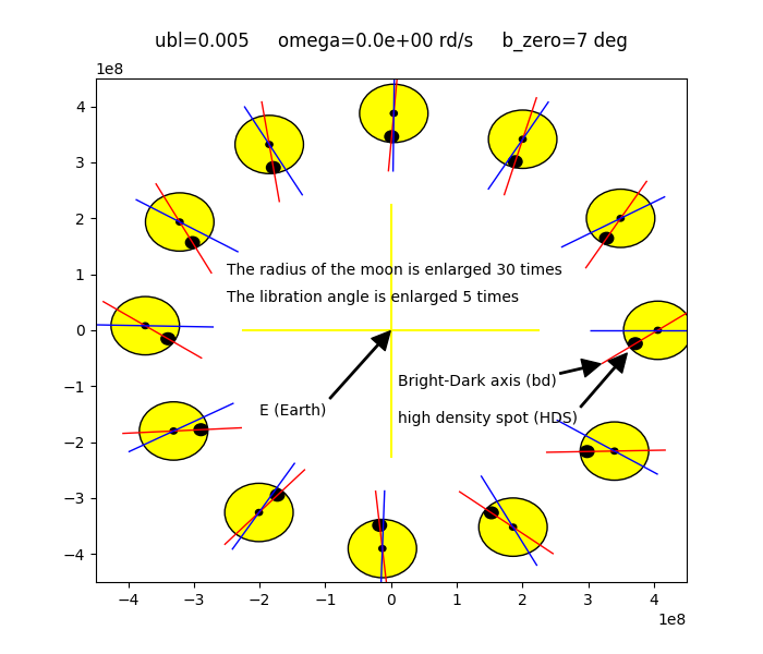
In “libration” mode
The program simulates the pendulum effect in an idealized case where the tidal effect is assumed to be zero and where the mass imbalance ubl is concentrated at a single point, the HDS (High Density Spot), located at point N (Nearest, origin of selenographic coordinates).
The initial pendulum angle is set to 7 degrees, and ubl is then varied at each run until the best match with reality is obtained, namely one full pendulum swing per orbit.
This result is reached for ubl = 5 per thousand, where the following figure is obtained:
In “rotation” mode
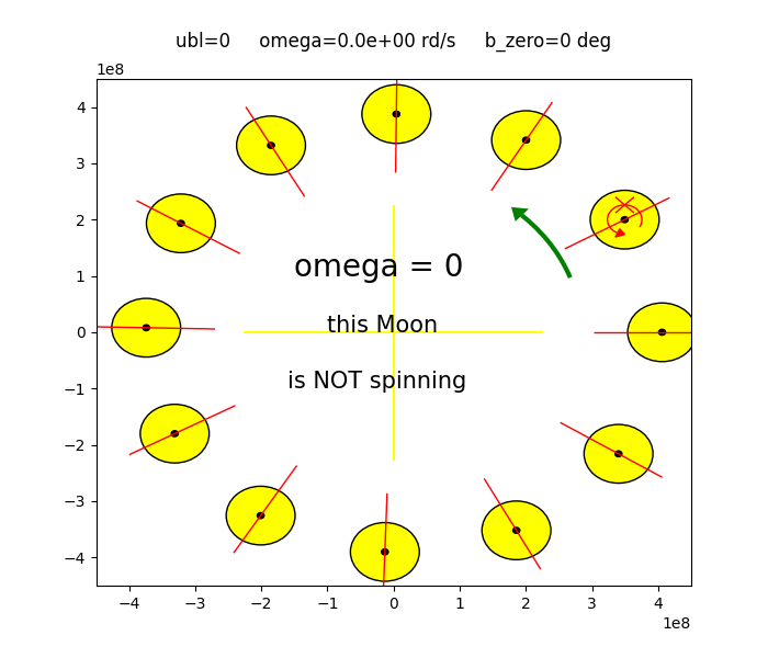
All libration effects are cancelled, which makes it possible to simulate the continuous rotation(s) of the Moon as seen in the left‑hand or right‑hand figures on the site https://science.nasa.gov/moon/tidal-locking/ (these figures appear almost identically on https://en.wikipedia.org/wiki/Tidal_locking).
left‑hand figure (“real” Moon)
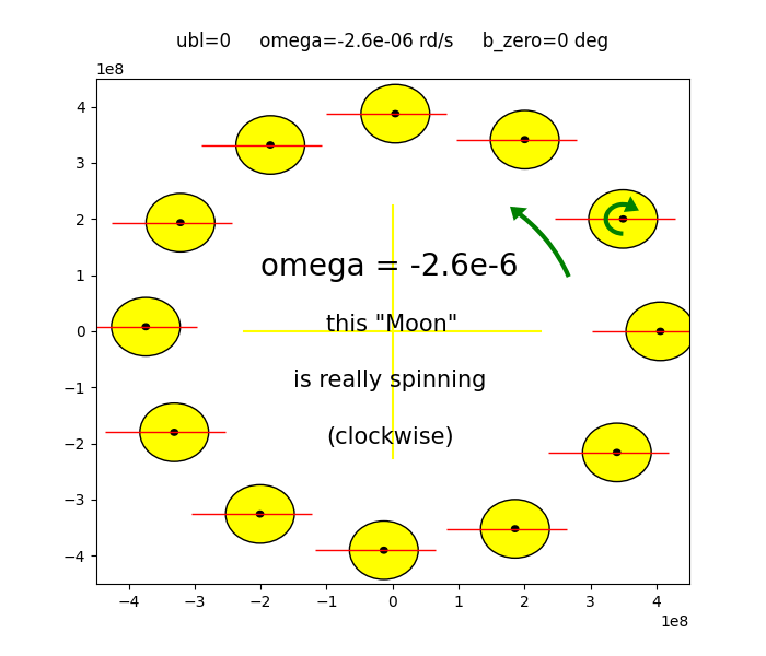
right‑hand figure (“false” Moon)
The two figures allow us to confirm, through dynamics, the result already obtained through geometry, namely the validity of the NSM design and the unreality of the SM design. It is indeed when executed with an angular velocity omega of zero that the program generates the “true” Moon on the left.
It generates the “false” Moon on the right when omega corresponds to a value opposite to the angular velocity of the orbit, that is -2.6e-6 rad/s.
The code below displays and runs perfectly once copied directly into Sublime Text or VS Code.
Code
# coding = utf - 8


"""
                           ********************************************************
                           * SIMULATION OF THE LONGITUDINAL LIBRATION OF THE MOON *
						   *				   February 28, 2022 				  *
                           ********************************************************

                           						Gilbert Vidal

                            Minor updates: on March 20, 2023 and Decembre 10, 2024


No entries.
Change any parameter directly in its declaration.
If you do so, don't forget to register before running.


A vector begins with an upper case letter.
The unit vector of an axis begins with the upper case U.
The vector from B to C is labelled BC. But, as E is the origin, the vector EC is labelled C.
A scalar begins with a lower case letter.
The coordinates of the point P are those of the vector EP (because E is the origin of the plan).
The distance between the points B and C is labelled lBC (l stands for length).
The angles are expressed  1/ in radians for calculations
                          2/ in degrees for inputs/outputs (with suffix _d).

"""

import numpy as np
from math import cos, sin, radians, degrees, sqrt, pi
import matplotlib.pyplot as plt
from matplotlib.patches import Arc, Polygon, Circle


#1 - choose mode libration or rotation
mode = 0											#0: rotation mode		1: libration mode

#2 - choose figure left or right (no incidence if mode == 1)
rotation = "right"									#"left": related to the left animated figure
													#"right": related to the right animated figure

omega = 0 											#angular velocity of the Moon around
													#its centre of mass (rd/s)
if rotation == "right" and mode == 0:
	omega = -2*pi/(28*24*3600)


#VECTORIAL FUNCTIONS *********************************************************************************

def sum(V0,V1):                                    #sum of vectors V0 and V1
    return V0[0] + V1[0], V0[1] + V1[1]
def dif(V0,V1):                                     #sum of vectors V0 and V1
    return V0[0] - V1[0], V0[1] - V1[1]
def mod(V):                                         #module of the vector V
    return sqrt(V[1]**2 + V[0]**2)
def dist(V0, V1):
    return mod(dif(V0, V1))                         #distance entre 2 points
def kV(k, V0):                                      #product of vector V0 by a scalar k
    return k*V0[0], k*V0[1]
def Vecprod(V0, V1):                                #scalar of the vectorial product of vectors V0 and V1
    return V0[0]*V1[1] - V0[1]*V1[0]
def unit(V0, V1):                                   #unitary Vector of an axis bearing (parallel to)
    V = dif(V1,V0)                                     #the vector P0P1 (= (V1 - V0))
    return kV(1/mod(V), V)
def rot(ori, ext, angle):                           #Rotation du POINT ext d’un angle (en degrés) autour de ori
    a = radians(angle)
    V = dif(ext, ori)
    x, y = V                                        #retourne un point, pas un vecteur
    return sum(ori, (x*cos(a) - y*sin(a), x*sin(a) + y*cos(a)))


#UNIVERSAL CONSTANTS  *********************************************************************

r = 1.737e6                         #radius of the Moon (m)
mass = 7.34e22                      #mass of the Moon (kg)
mass_earth = 5.97e24                #mass of the Earth (kg)
g = 6.673e-11                       #gravitational constant  N·(m/kg)
v_zero = 970                        #velocity of the Moon at start (m/s)
lEC_zero = 4.06e8                   #Distance (length) at start between the mass centre C
                                    #    of the Moon and the Earth M (at apogee).
                                    #As regards the distance between Earth and Moon,
                                    #    EC and EM are supposed equal.

                                    #https://en.wikipedia.org/wiki/Lunar_distance_(astronomy)
                                    #from 356,500 km at the perigee to 406,700 km at apogee,
                                    #https://nssdc.gsfc.nasa.gov/planetary/factsheet/moonfact.html
                                        #Perigee            3.63e8
                                        #Apogee              4.06e8  **************
                                        #Max. orbital velocity     1082
                                        #Min. orbital velocity (km/s)    0.970  **********
                                        #revolution period (days)    27.3217


#CONSTANTS *********************************************************************************

ubl = + .005                        #relative unbalance due to the HDS (high density spot)
if mode == 0: ubl = 0
mass_s = ubl*mass                   #mass of the HDS
da = .01                            #angular orbital increment of a sample (rd)
b_zero_d = 7						#pendulum angle of the Moon at start IN DEGREES
if mode == 0: b_zero_d = 0
b_zero = b_zero_d*pi/180            #pendulum angle of the Moon at start (in rd of course)

m = mass_s*r/(mass)                 #abciss on the axis bd of the geographic centre of the moon
                                    #bd is the relative axis joining the bright and dark poles.
                                    #bd is oriented from bright pole to dark pole.
                                    #Its origin is C, center of mass of the Moon.

s = - r                             #abciss on the bd axis of the HDS

MoI = mass*r**2*(1 + ubl)           #moment of inertia (relative to C) of the Moon


#INITIALIZATION OF THE VARIABLES   ********************************************************

a = 0                               #orbital angle (rd)
b = b_zero                          #pendulum angle (rd)
if mode == 0: b = 0
db = 0							    #angular increment (for display purposes)
C = [lEC_zero, 0]                   #vector EC (coordinates of the centre of mass of the Moon (m))
V = [0, v_zero]                     #coordinates of the vector velocity of the centre of mass (m/s)
t = 0                               #time
dt = da*lEC_zero/v_zero             #duration of the orbital increment of a sample.
                                    #dt is not constant. This is only its initialization value.
                                    #dt is NOT the increment of the main loop.
                                    #dt is calculated at each loop. The true increment is angle da.
nb_samp_total = int(2*pi/da)        #number of samples of the MAIN LOOP
nb_plots = 12                       #number of plots of the MAIN LOOP
nb_samp_between_plots = int(nb_samp_total/nb_plots)          #number of samples between 2 plots
num = 0								#number of the current plot (for display purposes)


#FOR VISUALIZATION NEEDS ******************************************************************

kb = 5                              #ampli factor applied on the pendulum angle for visu needs
if mode == 0: kb = 1
kr = 30                             #ampli factor applied on the radius for visu needs
r_v = kr*r							#radius of the visualized Moon
rspot_v	= r_v/5						#radius of the visualized HDS (High Density Spot)
									#(the real HDS has no radius. It is infinitely small)

s_v = -r_v + rspot_v				#abcissis on the bd axix of the centre of the visualized HDS


#GRAPHICS  (except the plotting of the Moon itself)*****************************************

fig = plt.figure(figsize=(7, 6))	#total size: 7 by 6 inches
ax = fig.add_subplot(1,1,1)

xy = 450e6
xmin =  - xy  ;  xmax = xy  ;  ymin =  - xy  ;  ymax = xy
s1="{:.1e}".format(omega)
titre1 = 'ubl=' + str(ubl) + '     omega=' + s1 + ' rd/s' + '     b_zero=' + str(b_zero_d) + ' deg' + '\n'
ax.set(xlim = (xmin, xmax), ylim = (ymin, ymax), title = titre1)
plt.plot([xmin/2, xmax/2], [0,0], color='yellow')  ;  plt.plot([0,0], [ymin/2, ymax/2], color='yellow')

def annot(txt, xy, xytext):
	ax.annotate(txt, xy, xytext, arrowprops=dict(facecolor='black', shrink=0.01, width=1))
def annot1(txt, xy, size):#**kwargs):
	ax.annotate(txt, xy, size=size)

if mode == 1:
	annot('E (Earth)', (0, 0), (-2e8, -1.5e8))
	annot1('The radius of the moon is enlarged ' + str(kr) + ' times', (-2.5e8, 1e8), size=10)
	annot1('The libration angle is enlarged ' + str(kb) + ' times', (-2.5e8, .5e8), size=10)
	annot('Bright-Dark axis (bd)', (3.2e8, -.6e8), (.1e8, -1e8))
	annot('high density spot (HDS)', (3.6e8, -.4e8), (.1e8, -1.65e8))
if mode == 0:
	if rotation == "left":
		annot1('omega = 0', (-1.5e8, 1e8), size=20)
		annot1('this Moon', (-1e8, 0), size=15)
		annot1('is NOT spinning', (-1.6e8, -1e8), size=15)
	if rotation == "right":
		annot1('omega = -2.6e-6', (-2e8, 1e8), size=20)
		annot1('this "Moon"', (-1e8, 0), size=15)
		annot1('is really spinning', (-1.5e8, -1e8), size=15)
		annot1('(clockwise)', (-1e8, -2e8), size=15)

def flèche(C, Pf, direction, k, color, lw):  #Flèche triangulaire, pointe en bout de l'arc_gv coté a2.

    #construire le milieu B de la base de la flèche en faisant tourner Pf d'un petit angle a autour de C.
    #Puis construire Q1 ET Q2 sur le rayon CB
    #k: facteur pour passser des dimensions en carreaux de grille à celles pour le calcul

    r = dist(C, Pf)           #rayon de la flèche
    l_encarreau = .1          #longueur de la flèche en carreaux de grille
    l = l_encarreau*k         #longueur de la flèche
    a = degrees(l/r)          #angle de rotation donnant la longueur de la flèche
    b_encarreau = .07         #demi-base de la flèche en carreaux de grille
    b = b_encarreau*k         #demi-base de la flèche
    B = rot(C, Pf, -1*direction*a)
    U = unit(B, C)
    Q1 = sum(B, kV(-b, U)) ; Q2 = sum(B, kV(b, U))
    points = (Q1, Pf, Q2)
    arro = Polygon(points, color=color, lw=lw)
    ax.add_patch(arro)
    fig.canvas.draw_idle()
    return arro

def arc_gv(C, r, a1, a2, direction, k,color, lw): #C: centre, r: rayon, a1, a2: angles de début et de fin de l'arc en degrés, lw: épaisseur de l'arc
    cx, cy = C
    Pf = rot(C, (cx + r, cy), a2)  #point de fin de l'arc
    if direction < 0: a1, a2 = a2, a1
    arc = Arc((cx, cy), 2*r, 2*r,
                angle=0, theta1=a1, theta2=a2, color=color, lw=lw)
    ax.add_patch(arc)
    fig.canvas.draw_idle()
    return arc_gv, (C, Pf, direction, k, color, lw)

def X_gv(ax, Xrouge, L, angle_deg, color='red', lw=2, **kwargs):
    #dans polygon je peux mettre directement le point P, pas dans line2D
    P_0=sum(Xrouge, (L, 0))
    A1 = rot((Xrouge), P_0, angle_deg) ; A2 = rot((Xrouge), P_0, -angle_deg)
    B1 = rot((Xrouge), P_0, angle_deg + 180) ; B2 = rot((Xrouge), P_0, -angle_deg + 180)
    pol1 = Polygon((A1, B1), color=color, lw=lw, **kwargs); ax.add_patch(pol1)
    pol2 = Polygon((A2, B2), color=color, lw=lw, **kwargs) ; ax.add_patch(pol2)


#Grande flèche verte
arc, args_fleche = arc_gv((0,0), .70*lEC_zero, 20, 50, 1, xy/4, 'green', 3)
flèche(*args_fleche)


#MAIN LOOP  The increment is da, it is not dt*****************************************
#           ********************************************************************************


output = 0

for i_sample in range(nb_samp_total):


	def mapping():

		global lEC, lEB, Ue, Ufs, Ubd, M, Ubd_v, B, CB, a, b

		if  mode == 0 and rotation == "right":
			pass
			b = -a		# This line is a deliberate cheating to display the ideal expected result.
						# Comment it out (replace 'b' with '#b') if you want to highlight
						# the real figure.

		Ue = (cos(a), sin(a))                     #unitary vector on the axis EM
		Ubd = (cos(a + b), sin(a + b))            #unitary vector on the axis bd
		Ubd_v = (cos(a + kb*b), sin(a + kb*b))      #unitary vector on the axis bd "magnified" (displayed)
		E = (0, 0)							#centre of the Earth
		M = C                              	#centre of the Moon,
											#it is assumed to coincide with the center of mass
		CB = kV(s, Ubd)                     	#vector CB
		B = sum(C, CB)                     	#vector EB: coordinates of the point B
		Ufs = unit(B, E)				   	#unitary vector of the attractive force due to the HDS.
		lEC = mod(C)                       	#distance between the Earth and the centre of mass of the Moon
		lEB = mod(B)                       	#distance between the Earth and the HDS (or B)


	mapping()


    #TRAJECTORY OF THE CENTRE OF MASS OF THE MOON

	f = g*mass*mass_earth/lEC**2
	F = kV(-f, Ue)
	V = sum(V, kV(dt/mass, F))
	C = sum(C, kV(dt, V))


    #PENDULUM MOVEMENT

	fs = g*mass_s*mass_earth/lEB**2     #module of the force exercised by the Earth on the HDS
	Fs = kV(fs, Ufs)                    #vector of the force exercised by the Earth on the HDS
	moment = Vecprod(kV(s, Ubd), Fs)     #scalar of the moment due to the HDS


    #OUTPUTS

	if (i_sample % nb_samp_between_plots  == 0) and (i_sample < (nb_samp_total -10)):

		MB_v = kV(s_v, Ubd_v)						#visualized vector MB
		B_v = sum(M, MB_v)                      #coordinates of the centre of the visualized HDS
		moon = Circle(M, r_v, alpha=1, facecolor="yellow", edgecolor="black")
		spot = Circle(B_v, rspot_v, alpha=1, color="black")
		centre = Circle(M, r_v/10, alpha=1, color="black")
		me1 = sum(M, kV(-2*r_v, Ue))  ;  me2 = sum(M, kV(1.5*r_v, Ue))
		bd1 = sum(M, kV(-2*r_v, Ubd_v))  ;  bd2 = sum(M, kV(1.5*r_v, Ubd_v))
		axis_me1 = (me1, me2)
		axis_bd1 = (bd1,bd2)
		axis_me = Polygon(axis_me1, color="blue")
		axis_bd = Polygon(axis_bd1, color="red")
		ax.add_artist(moon)
		#if mode == 1: ax.add_artist(spot)
		ax.add_artist(centre)
		ax.add_artist(axis_bd)
		if mode == 1: ax.add_artist(axis_me, spot)
		output = output + 1

		if output == 2: M2 = M

	mapping()


    #INCREMENTATIONS

	v_trajectory = sqrt(mod(V)**2)
	Proj = Vecprod(V, Ufs)				#projection of vector V on the perpendicular to Ufs
	dt = da*lEC/v_trajectory
	#dt = da*lEC/Proj
	omega = omega + moment*dt/MoI
	db = omega*dt
	a = a + da
	b = b + db
	t = t + dt


#ARCS AND ARROWS ON THE MOON IN THE ROTATION MODE

r_flèche = r*kr/2						#rayon de la petite flèche
if mode == 0 and rotation == "right":
	arc, args_fleche = arc_gv(M2, r_flèche, 270, 45, -1, xy/4, 'green', 3)
	flèche(*args_fleche)
if mode == 0 and rotation == "left":
	arc, args_fleche = arc_gv(M2, r_flèche, -30, 270, 1, 'red', 1)
	flèche(*args_fleche)
	Xrouge = (M2[0], M2[1] + r_flèche)
	X_gv(ax, Xrouge, 2e7, 45, color='red', lw=1)


#FINAL

days = t / (24*3600)
print ('\n', i_sample, '   ', 'v0=', v_zero, '    ', 'total time=', '%.2f' % days,'days')

plt.show()
