Libration

Présentation et résultats

La Lune présente un mouvement oscillatoire autour de son axe principal, d’une amplitude d’environ 7 degrés, appelé libration longitudinale.
Dans la conception traditionnelle SM (Spinning Moon), on explique ce phénomène de manière cinématique, par la combinaison de l’excentricité de l’orbite lunaire et de sa supposée rotation sur elle‑même.

Dans la conception NSM (Non‑Spinning Moon), où cette rotation n’existe pas, la libration peut s’expliquer par la conjonction de deux effets dynamiques :

l’effet de marée bien connu ¹, présenté par exemple dans https://fr.wikipedia.org/wiki/Rotation_synchrone
un effet jamais étudié auparavant, que nous appellerons effet culbuto², dû à un léger déséquilibre de masse en faveur de l’hémisphère faisant face à la Terre.

¹ Dans NSM l’effet de marée est bien réel, alors que la rotation synchrone n’existe pas.
²Les effets de marée et culbuto se traduisent tous deux par un mouvement pendulaire.

Le programme dont le code source est fourni ci‑dessous peut s’exécuter selon deux modes : un mode principal appelé «libration», et un mode auxiliaire appelé «rotation».

Grâce à la bibliothèque Matplotlib, l’image de la Lune est ajoutée au tracé à intervalles angulaires réguliers, et l’image finale en fin d’orbite est restituée à la fin du programme.

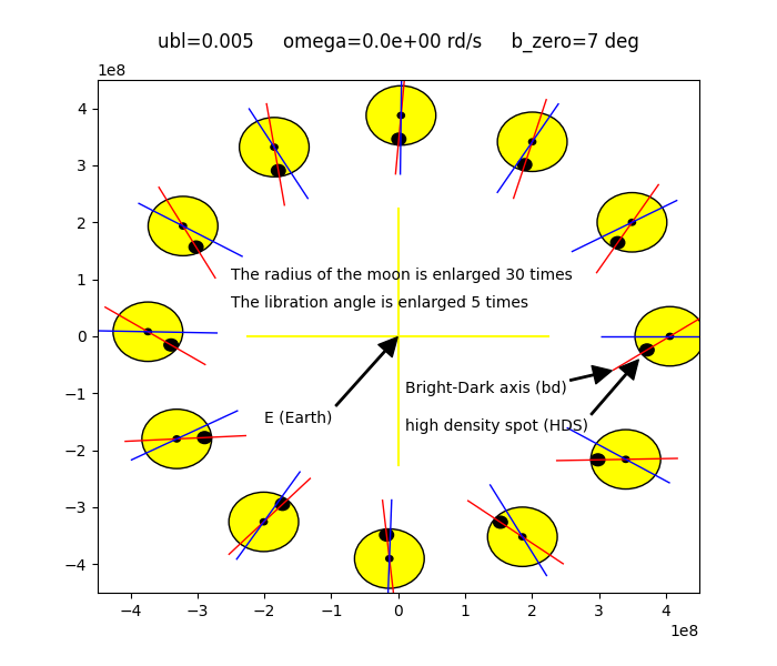
En mode “libration”

Le programme simule l’effet pendulaire dans un cas d’école où l’effet de marée est supposé nul et où le déséquilibre de masse ubl est concentré en un seul point, le HDS (High Density Spot), situé au point N (Nearest, origine des coordonnées sélénographiques).
On fixe l’angle pendulaire initial à 7 degrés, puis on fait varier ubl à chaque exécution jusqu’à obtenir la meilleure correspondance avec la réalité, c’est‑à‑dire un battement pendulaire complet par orbite.
On constate que ce résultat est atteint pour ubl = 5 pour mille, où on obtient la figure suivante :

En mode «rotation»

Tout effet de libration est annulé ce qui permet de simuler la ou les rotations continues de la Lune telles que l’on peut les voir dans les figures de gauche ou de droite du site https://science.nasa.gov/moon/tidal-locking/ (on retrouve ces figures pratiquement à l’dentique dans le site https://fr.wikipedia.org/wiki/Rotation_synchrone).

figure de gauche (“vraie” Lune)

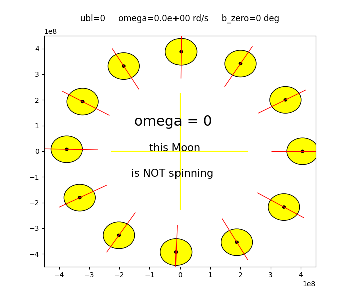
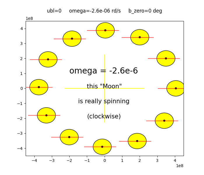
figure de droite (“fausse” Lune)

Les deux figures permettent de confirmer par la dynamique le résultat déjà obtenu par la géométrie, à savoir la validité de la conception NSM et l’irréalité de la conception SM. C’est bien quand il est exécuté avec une vitesse angulaire omega nulle que le programme génère la “vraie” Lune de gauche.
Il génère la “fausse” lune de droite lorsque omega correspond à une valeur opposée à la vitesse angulaire de l’orbite, soit -2.6e-6 rd/s.

Code

			
Le code ci-dessous se présente et s'exécute parfaitement une fois copié
directement dans Sublime Text ou VS Code (je n'ai pas testé d'autres éditeurs).
# coding = utf - 8
"""
                           ********************************************************
                           * SIMULATION OF THE LONGITUDINAL LIBRATION OF THE MOON *
						   *				   February 28, 2022 				  *	
                           ********************************************************
                           						Gilbert Vidal
                            Minor updates: on March 20, 2023 and Decembre 10, 2024
                           
No entries.
Change any parameter directly in its declaration.
If you do so, don't forget to register before running.
A vector begins with an upper case letter.
The unit vector of an axis begins with the upper case U.
The vector from B to C is labelled BC. But, as E is the origin, the vector EC is labelled C.
A scalar begins with a lower case letter.
The coordinates of the point P are those of the vector EP (because E is the origin of the plan).
The distance between the points B and C is labelled lBC (l stands for length).
The angles are expressed  1/ in radians for calculations
                          2/ in degrees for inputs/outputs (with suffix _d).
"""
import numpy as np
from math import cos, sin, radians, sqrt, pi
import matplotlib.pyplot as plt
import matplotlib.lines as lines
import matplotlib.path as path
import matplotlib.patches as patches
#1 - choose mode libration or rotation
mode = 0											#0: rotation mode		1: libration mode
#2 - choose figure left or right (no incidence if mode == 1)
rotation = "left"									#"left": related to the left animated figure
													#"right": related to the right animated figure
omega = 0 											#angular velocity of the Moon around
													#its centre of mass (rd/s)
if rotation == "right" and mode == 0:
	omega = -2*pi/(28*24*3600)
#VECTORIAL FUNCTIONS *********************************************************************************
def sum(V0,V1):                                     #sum of vectors V0 and V1
    return V0[0] + V1[0], V0[1] + V1[1]
def dif(V0,V1):                                     #sum of vectors V0 and V1
    return V0[0] - V1[0], V0[1] - V1[1]
def mod(V):                                         #module of the vector V
    return sqrt(V[1]**2 + V[0]**2)                         
def kV(k, V0):                                      #product of vector V0 by a scalar k
    return k*V0[0], k*V0[1]
def Vecprod(V0, V1):                                #scalar of the vectorial product of vectors V0 and V1
    return V0[0]*V1[1] - V0[1]*V1[0]
def unit(V0, V1):                                   #unitary Vector of an axis bearing (parallel to)
    V = dif(V1,V0)                                     #the vector P0P1 (= (V1 - V0))
    return kV(1/mod(V), V) 
#UNIVERSAL CONSTANTS  *********************************************************************
r = 1.737e6                         #radius of the Moon (m)               
mass = 7.34e22                      #mass of the Moon (kg)
mass_earth = 5.97e24                #mass of the Earth (kg)
g = 6.673e-11                       #gravitational constant  N·(m/kg)
v_zero = 970                        #velocity of the Moon at start (m/s)
lEC_zero = 4.06e8                   #Distance (length) at start between the mass centre C
                                    #    of the Moon and the Earth M (at apogee).
                                    #As regards the distance between Earth and Moon,
                                    #    EC and EM are supposed equal.
                                    
                                    #https://en.wikipedia.org/wiki/Lunar_distance_(astronomy)
                                    #from 356,500 km at the perigee to 406,700 km at apogee, 
                                    #https://nssdc.gsfc.nasa.gov/planetary/factsheet/moonfact.html
                                        #Perigee            3.63e8
                                        #Apogee              4.06e8  **************
                                        #Max. orbital velocity     1082 
                                        #Min. orbital velocity (km/s)    0.970  **********
                                        #revolution period (days)    27.3217
                                
#CONSTANTS *********************************************************************************
ubl = + .005                        #relative unbalance due to the HDS (high density spot)
if mode == 0: ubl = 0
mass_s = ubl*mass                   #mass of the HDS
da = .01                            #angular orbital increment of a sample (rd)
b_zero_d = 7						#pendulum angle of the Moon at start IN DEGREES
if mode == 0: b_zero_d = 0
b_zero = b_zero_d*pi/180            #pendulum angle of the Moon at start (in rd of course)
                  
m = mass_s*r/(mass)                 #abciss on the axis bd of the geographic centre of the moon 
                                    #bd is the relative axis joining the bright and dark poles.
                                    #bd is oriented from bright pole to dark pole.
                                    #Its origin is C, center of mass of the Moon.    
s = - r                             #abciss on the bd axis of the HDS
MoI = mass*r**2*(1 + ubl)           #moment of inertia (relative to C) of the Moon
#INITIALIZATION OF THE VARIABLES   ********************************************************
a = 0                               #orbital angle (rd)
b = b_zero                          #pendulum angle (rd)
if mode == 0: b = 0
db = 0							    #angular increment (for display purposes)
C = [lEC_zero, 0]                   #vector EC (coordinates of the centre of mass of the Moon (m))
V = [0, v_zero]                     #coordinates of the vector velocity of the centre of mass (m/s)
t = 0                               #time
dt = da*lEC_zero/v_zero             #duration of the orbital increment of a sample.
                                    #dt is not constant. This is only its initialization value.     
                                    #dt is NOT the increment of the main loop.
                                    #dt is calculated at each loop. The true increment is angle da.
nb_samp_total = int(2*pi/da)        #number of samples of the MAIN LOOP
nb_plots = 12                       #number of plots of the MAIN LOOP
nb_samp_between_plots = int(nb_samp_total/nb_plots)          #number of samples between 2 plots
num = 0								#number of the current plot (for display purposes)	
#FOR VISUALIZATION NEEDS ******************************************************************
kb = 5                              #ampli factor applied on the pendulum angle for visu needs
if mode == 0: kb = 1		
kr = 30                             #ampli factor applied on the radius for visu needs
r_v = kr*r							#radius of the visualized Moon
rspot_v	= r_v/5						#radius of the visualized HDS (High Density Spot)
									#(the real HDS has no radius. It is infinitely small)
s_v = -r_v + rspot_v				#abcissis on the bd axix of the centre of the visualized HDS
#GRAPHICS  (except the plotting of the Moon itself)*****************************************
fig = plt.figure(figsize=(7, 6))	#total size: 7 by 6 inches
ax = fig.add_subplot(1,1,1)
    
xy = 450e6
xmin =  - xy  ;  xmax = xy  ;  ymin =  - xy  ;  ymax = xy
s1="{:.1e}".format(omega)
titre1 = 'ubl=' + str(ubl) + '     omega=' + s1 + ' rd/s' + '     b_zero=' + str(b_zero_d) + ' deg' + '\n'
ax.set(xlim = (xmin, xmax), ylim = (ymin, ymax), title = titre1)
plt.plot([xmin/2, xmax/2], [0,0], color='yellow')  ;  plt.plot([0,0], [ymin/2, ymax/2], color='yellow')
def annot(txt, xy, xytext):
	ax.annotate(txt, xy, xytext, arrowprops=dict(facecolor='black', shrink=0.01, width=1))
def annot1(txt, xy, size):#**kwargs):
	ax.annotate(txt, xy, size=size)
if mode == 1:
	annot('E (Earth)', (0, 0), (-2e8, -1.5e8))
	annot1('The radius of the moon is enlarged ' + str(kr) + ' times', (-2.5e8, 1e8), size=10)
	annot1('The libration angle is enlarged ' + str(kb) + ' times', (-2.5e8, .5e8), size=10)
	annot('Bright-Dark axis (bd)', (3.2e8, -.6e8), (.1e8, -1e8))
	annot('high density spot (HDS)', (3.6e8, -.4e8), (.1e8, -1.65e8))
if mode == 0:
	if rotation == "left":
		annot1('omega = 0', (-1.5e8, 1e8), size=20)		
		annot1('this Moon', (-1e8, 0), size=15)
		annot1('is NOT spinning', (-1.6e8, -1e8), size=15)
	if rotation == "right":
		annot1('omega = -2.6e-6', (-2e8, 1e8), size=20)		
		annot1('this "Moon"', (-1e8, 0), size=15)
		annot1('is really spinning', (-1.5e8, -1e8), size=15)
		annot1('(clockwise)', (-1e8, -2e8), size=15)
		
#MAIN LOOP  The basic increment is da, it is not dt*****************************************
#           ********************************************************************************
 
for i_sample in range(nb_samp_total):
    
	def mapping():
	
		global lEC, lEB, Ue, Ufs, Ubd, M, Ubd_v, B, CB, a, b
		
		if  mode == 0 and rotation == "right":
			pass
			b = -a		# This line is a deliberate cheating to display the ideal expected result.
						# Comment it out (replace 'b' with '#b') if you want to highlight
						# the real figure.
		
		Ue = (cos(a), sin(a))                     #unitary vector on the axis EM   
		Ubd = (cos(a + b), sin(a + b))            #unitary vector on the axis bd
		Ubd_v = (cos(a + kb*b), sin(a + kb*b))      #unitary vector on the axis bd "magnified" (displayed)
		E = (0, 0)							#centre of the Earth
		M = C                              	#centre of the Moon,
											#it is assumed to coincide with the center of mass
		CB = kV(s, Ubd)                     	#vector CB 
		B = sum(C, CB)                     	#vector EB: coordinates of the point B
		Ufs = unit(B, E)				   	#unitary vector of the attractive force due to the HDS.	
		lEC = mod(C)                       	#distance between the Earth and the centre of mass of the Moon
		lEB = mod(B)                       	#distance between the Earth and the HDS (or B)	
    
	   
	mapping()
 
    #TRAJECTORY OF THE CENTRE OF MASS OF THE MOON
    
	f = g*mass*mass_earth/lEC**2 
	F = kV(-f, Ue)
	V = sum(V, kV(dt/mass, F))
	C = sum(C, kV(dt, V))
    #PENDULUM MOVEMENT
	fs = g*mass_s*mass_earth/lEB**2     #module of the force exercised by the Earth on the HDS
	Fs = kV(fs, Ufs)                    #vector of the force exercised by the Earth on the HDS
	moment = Vecprod(kV(s, Ubd), Fs)     #scalar of the moment due to the HDS
	
    #OUTPUTS
	if (i_sample % nb_samp_between_plots  == 0) and (i_sample < (nb_samp_total -10)):
		
		MB_v = kV(s_v, Ubd_v)						#visualized vector MB 
		B_v = sum(M, MB_v)                      #coordinates of the centre of the visualized HDS
		moon = patches.Circle(M, r_v, alpha=1, facecolor="yellow", edgecolor="black")
		spot = patches.Circle(B_v, rspot_v, alpha=1, color="black")
		centre = patches.Circle(M, r_v/10, alpha=1, color="black")
		me1 = sum(M, kV(-2*r_v, Ue))  ;  me2 = sum(M, kV(1.5*r_v, Ue))
		bd1 = sum(M, kV(-2*r_v, Ubd_v))  ;  bd2 = sum(M, kV(1.5*r_v, Ubd_v))
		axis_me1 = (me1, me2)
		axis_bd1 = (bd1,bd2)
		axis_me = patches.Polygon(axis_me1, color="blue")
		axis_bd = patches.Polygon(axis_bd1, color="red")
		ax.add_artist(moon)
		if mode == 1: ax.add_artist(spot)
		ax.add_artist(centre)
		ax.add_artist(axis_bd)
		if mode == 1: ax.add_artist(axis_me)
		
	mapping()
    
   
    #INCREMENTATIONS
    
	v_trajectory = sqrt(mod(V)**2)
	Proj = Vecprod(V, Ufs)				#projection of vector V on the perpendicular to Ufs
	dt = da*lEC/v_trajectory
	#dt = da*lEC/Proj
	omega = omega + moment*dt/MoI
	db = omega*dt
	a = a + da
	b = b + db
	t = t + dt
	
 
#FINAL
days = t / (24*3600)
print ('\n', i_sample, '   ', 'v0=', v_zero, '    ', 'total time=', '%.2f' % days,'days')
plt.show()

		

Gilbert Vidal — retired engineer (France)